 The Joy of Cryptography
Modern Computational Cryptography
Imagine an encryption scheme that can be broken, but the fastest possible attack requires a trillion years of computation. You probably wouldn't worry about such an attack because there is no meaningful difference between a task that takes a trillion years and a task that is simply impossible. But our style of security definitions is completely agnostic to an attack's running time. If there is a calling program that can distinguish two libraries after a trillion years of computation, then those libraries are deemed not interchangeable. An encryption scheme that allows this kind of attack would be deemed insecure.
Now imagine an encryption scheme that can be broken, but the best possible attack is guaranteed to succeed only with extremely low probability. In fact, the probability that the attack succeeds is smaller than the probability of winning the lottery a hundred times in a row. Again, you probably wouldn't worry about this attack because there is no meaningful difference between an event that happens with such a tiny probability and an event that is simply impossible. But our style of security definitions is completely agnostic to an attack's success probability. If there is a calling program that can distinguish two libraries, with output probabilities that are different by the tiniest nonzero amount, then those libraries are deemed not interchangeable. An encryption scheme that allows this kind of attack would be deemed insecure.
The modern approach to provable security builds on the vocabulary that we developed in chapter 2 but dismisses attacks with astronomically high computational cost or astronomically tiny success probability. Instead of proving statements like: No attack against this scheme can succeed at all, not even in principle, we will prove statements like: Every attack against this scheme has either astronomically high computational cost or astronomically small success probability.
We'll start by clarifying precisely what is meant by “astronomically” high costs or low probabilities.
4.1. The concrete approach to provable security
In the concrete approach to provable security, our goal is to be as quantitative as possible about security claims. We rarely say definitively that a cryptographic algorithm “is secure,” as we did when discussing OTP. Instead, we say things like, “any attack that expends at most effort can succeed with probability no better than .” It is up to the user to judge whether this quantitative level of security is acceptable, based on their use-case and risk tolerance.
4.1.1. Huge numbers
The concrete approach requires good intuition about huge numbers (like ) and tiny numbers (like ). Here are some examples to help put huge computations into perspective:
One way to think about huge computations is their monetary cost. Below, I have calculated roughly how much a computation involving CPU cycles would cost on the cheapest available Amazon EC2 cloud computing service:
| cycles | approx cost (USD) | point of reference |
| $3.50 | cup of coffee | |
| $100 | good tickets to a Portland Trailblazers game | |
| $130,000 | median home price in Chickasaw County, Iowa | |
| $130 million | budget of one of the Harry Potter movies | |
| $140 billion | GDP of Hungary | |
| $20 trillion | GDP of the United States | |
| $2 quadrillion | all of human economic activity since 300,000 bce | |
| a lot! | a billion human civilizations' worth of effort |
I don't intend to discuss cryptocurrencies much in this book. Let's just say that cryptocurrencies based on proof-of-work, like Bitcoin, incentivize their users to perform truly obscene amounts of computation. In Bitcoin's proof-of-work mechanism, users race to perform SHA-256 hash computations as fast as possible (it's not important to know what SHA-256 is for this illustration). At the time of writing, the collective Bitcoin network has performed approximately SHA-256 hashes in total, including in the last twelve months. The current market cap for Bitcoin is approximately 400 billion USD.
These two examples provide different monetary estimates because Bitcoin mining happens exclusively on special-purpose hardware (ASICs), which can perform Bitcoin mining and do nothing else. Cloud computing services offer general-purpose CPUs, which are orders of magnitude slower and less energy efficient, hence more expensive.
4.1.2. Tiny numbers
Next are some examples to help put tiny probabilities into perspective:
In the casino game called craps, the gambler rolls a pair of six-sided dice, and loses their bet if the dice add to 7. (This is a great oversimplification.) In 2009, Patricia Demauro rolled 154 consecutive times without getting a 7. This is arguably the most unlikely event ever recorded, with a probability of .
I can't find a reliable primary source, but many websites claim that the longest streak in roulette happened in 1943, when a gambler spun red 32 times in a row. The probability of spinning the same color 32 times in a row is (the first spin doesn't matter, but the next 31 must match).
The chance of winning the jackpot in the American Powerball lottery is . The chance of winning the Powerball on two consecutive weeks is .
This square is approximately 25 square millimeters, or about of the surface area of the Earth. If an alien throws a dart toward the Earth from a distant solar system, then with probability the dart will land exactly in the black square in your copy of The Joy of Cryptography.
There are roughly eight billion people on earth. If every one of them uniformly sampled an 80-bit string once per second, nonstop for a million years, then it is more than likely no one ever sampled the all-zeros string. There would have been “only” attempts in that time.
I encourage you to explore your own ways of understanding extreme numbers.
A computation taking steps will never happen in this universe. An event with probability less than is effectively impossible.
The last point about probability deserves some clarification.
-
Events with probability happen all the time. Every time you shuffle a deck of fifty-two cards, the probability of getting that particular ordering of the cards is approximately . The event that I describe as effectively impossible is that you have a specific ordering in mind before you shuffle, and then observe that ordering after shuffling. In cryptography we are always talking about specific events that are defined a priori. These are effectively impossible if their probability is .
-
You must take care to consider the probability of the correct event. There may be an encryption scheme that fails catastrophically (i.e., perhaps it completely leaks the secret key) with probability each time the algorithm is called. However, some attack scenarios might allow the algorithm to be invoked many times, giving an adversary many chances to trigger this catastrophic event. Of course, the adversary will be satisfied if any one of those chances succeed, so that is the event whose probability is most important. If an adversary causes to be called times, then the event that really matters happens not with probability but more like , which is “only” one in a billion.
It is often useful to think about a trade-off between an attack's running time and its success probability:
A cryptographic construction has bits of security (informally) if every attack satisfies the following relationship:
where “cost of attack” is measured in some low-level unit like CPU cycles or single-bit operations.
Typical cryptographic standards are designed to target at least 128 bits of security.
4.2. The asymptotic approach to provable security
The concrete approach is helpful for answering practical questions like, how large should my keys be to achieve a comfortable security level? But with that level of precision comes the responsibility of managing more tedious quantitative details during a security proof.
The asymptotic approach is an alternative that lets us make more qualitative, all-or-nothing statements, at the cost of losing some quantitative precision. “Asymptotic” means considering the behavior of an algorithm in the limit—that is, as the key size approaches infinity. You are probably familiar with asymptotic analysis using big- notation. Focusing only on asymptotic behavior allows us to hide many tedious quantitative details. For example, you don't need to carefully calculate that a certain operation takes exactly steps; you can stop as soon as you realize it takes steps.
A function is if there is a constant such that for all but finitely many values of . In other words, a constant multiple of eventually overtakes .
4.2.1. Polynomial running time
In the asymptotic approach, we only consider adversaries that run in polynomial time.
An algorithm runs in polynomial time if there is a polynomial such that the algorithm takes at most steps on inputs of length .
Cryptographic algorithms typically have several different inputs, so we always measure the running time as a function of the security parameter, which we write as Greek letter lambda . Usually, but not always, the security parameter is the length (in bits) of the secret keys in a cryptographic scheme. We assume that all algorithms and libraries have access to the value of as a global variable, although we don't write it as an explicit input.
Polynomial-time algorithms are closed under composition: A polynomial-time program that calls a polynomial-time subroutine can be combined into a monolithic algorithm whose overall running time is also polynomial. Without this composition property, many aspects of the theory would be problematic or incoherent.
4.2.2. Negligible probabilities
You've seen asymptotic analysis (big-) to categorize functions that approach infinity as their input grows, like the running time of an algorithm. Asymptotic analysis tells us how fast a function zooms off toward infinity.
In cryptography we also use asymptotic analysis to describe probabilities that approach zero as the input gets larger. We are interested in how fast these probability functions approach zero. If the probability of some event approaches zero fast enough, we can classify that event as effectively impossible.
Suppose a cryptographic algorithm fails catastrophically with probability . This probability clearly approaches zero as grows, but does it approach zero fast enough? There may be attack scenarios in which an adversary could have chances to trigger the catastrophic event, because is a polynomial, and we consider adversaries that have polynomial running time. With so many chances, the catastrophic event actually has a very good probability of happening in at least one of the attempts. Hence, does not seem to approach zero fast enough to ignore.
On the other hand, suppose the catastrophic failure happens with probability . If an adversary gets two chances to trigger the catastrophic event, it happens with probability at most ; if the adversary gets chances, the probability is at most . A polynomial-time adversary can get at most a polynomial number of chances to trigger the catastrophic event, but no matter what polynomial we place in the numerator, the denominator always “wins,” sending the overall probability to zero in the limit. Hence, approaches zero fast enough to be robust for polynomial-time situations.
In the asymptotic approach to cryptography, we require an adversary's success probability to approach zero faster than any reciprocal-polynomial. Formally:
A function is negligible if it approaches zero faster than , for every polynomial . There are a few ways to formalize this:
-
For every polynomial , there is a value such that for all . In other words, beyond , is always smaller than .
-
For every polynomial , we have . In case for some values of , we interpret as .
Here are a few examples of negligible functions:
-
is a negligible function because its reciprocal grows faster than all polynomials.
-
is negligible because also grows faster than all polynomials.
-
If is a polynomial, then is negligible.
Nearly every appearance of a negligible probability in this book will be easy to identify, usually having the form , where is some polynomial.
4.2.3. Comparing concrete vs asymptotic
In this book, we mostly stick to the asymptotic approach. The asymptotic style leads to simpler, cut-and-dry security statements like “every polynomial-time adversary succeeds with only negligible probability," whereas the concrete style demands that we carefully account for an adversary's advantage.
For example, a security theorem in the asymptotic style might read like this:
If is a secure PRF, then (which uses as a subroutine) is a CPA-secure encryption scheme.
It's not important right now to understand what “secure PRF” or “CPA-secure” means; these serve as merely an illustration here. The same theorem in the concrete style might read more like this:
For every calling program there exists a corresponding calling program , with similar runtime, such that:
where:
-
denotes the probability of successfully distinguishing the libraries from the CPA security definition for scheme . (This quantity is defined as 's advantage below.)
-
denotes the probability of successfully distinguishing the libraries from the PRF security definition for .
-
is the number of times calls its library.
Both the concrete and asymptotic approaches have clear merit, and both are common in the research literature. And it's important to acknowledge that everything we prove in this book in the asymptotic style could also be proven in a concrete style. Our fundamental approach of defining security in terms of libraries and distinguishers is compatible with both styles.
The concrete approach is necessary when determining proper key sizes. A security theorem in the asymptotic approach tells you only about a system's eventual behavior, in the limit as key sizes approach infinity. It tells you very little about its behavior for any specific key size.
Another important distinction between the concrete and asymptotic approaches is what happens if P = NP. For almost any cryptographic primitive, the problem of breaking it (asymptotically) is in the complexity class NP. So if P = NP, almost all of cryptography can be broken in polynomial time; asymptotic security is doomed in this case, but concrete security may still be viable.
4.3. Indistinguishability
In chapter 2, we said that two libraries were interchangeable if they induce identical output probabilities, for all adversaries. In the modern (asymptotic) approach, we say that two libraries are indistinguishable if they induce negligibly close output probabilities, for all polynomial-time adversaries:
Let and be two libraries with the same interface. If is a calling program, then the advantage of in distinguishing and is defined to be:
Libraries and are indistinguishable, written , if every polynomial-time calling program has only negligible advantage in distinguishing and . In other words, swapping for changes the behavior of a polynomial-time calling program by only a negligible amount.
Below are some facts about indistinguishability that are useful in security proofs:
For all polynomial-time libraries and :
-
If then
-
(transitivity) If then
-
(chain rule) If then
For (1), means that all calling programs—including the polynomial-time ones—have zero advantage distinguishing the libraries, and the constant function is indeed negligible. Thus, .
For (2) we can use two important facts:
-
If and are negligible functions, then is too (exercise 4.1).
-
(1-dimensional triangle inequality) If are real numbers, then .
Now, consider an arbitrary polynomial-time calling program and define , which is 's output probability when linked to . Now 's advantage distinguishing from is simply . But,
The last two terms are simply 's advantage distinguishing from , and its advantage distinguishing from , both of which we are assuming are negligible since . Hence 's advantage distinguishing from is negligible as well.
(3) is proven in essentially the same way as claim 2.4.1.
4.3.1. Hybrid proofs using indistinguishability
Indistinguishability is transitive, but there is an important subtlety: The negligible advantages “pile up.” Suppose , and suppose can't be distinguished from with advantage better than , as a function of the security parameter . Then, the advantage when distinguishing from could be as high as .
In simple security proofs like the ones we've seen so far, the number of hybrids does not depend on the security parameter, and everything works out as you might expect. The sum of a constant number of negligible functions is also negligible, and thus in the example above.
However, we will soon see proofs in which the number of hybrids depends on the security parameter. For example, in some upcoming proofs is the number of times the adversary calls the library. Since the adversary is assumed to run in polynomial time, is some unspecified polynomial function of the security parameter. These situations are more delicate, because the sum of a non-constant number of negligible functions might not be negligible (see exercise 4.3). Despite this, it is still possible to prove something like the following:
(Informally stated:) If and is a polynomial function of the security parameter, then .
Claim 4.3.3 is a simplification of the truth, but it captures the intuition needed to understand proofs later in this book: It is generally safe to write a proof with a polynomial number of hybrids.
You can safely stop at the informal statement of claim 4.3.3 if you prefer, but here are the gory details for those of you who are interested. It's not enough that (for all ), because this condition involves first fixing and then considering the libraries' asymptotic behavior as the security parameter approaches infinity. Instead, we must demand that , even against an adversary who can choose , because this new scenario allows to depend on the security parameter.
(Formal restatement of claim 4.3.3:) Let and be polynomial-time libraries. Suppose the following conditions hold:
-
“There are a polynomial number of hybrids, where the polynomial can depend on the calling program”: Formally, for every polynomial-time calling program , there exists a polynomial such that behaves exactly like , from the perspective of :
-
“Consecutive hybrids and are indistinguishable, even to an adversary who is allowed to choose the parameter .” Formally, the following two libraries are indistinguishable:
:if :become an instance of:if :become an instance ofWhen one of these libraries “becomes an instance” of , it means the library starts running the code of and behaving exactly like it in all respects. That is, it adopts the interface of and responds to subroutine calls exactly as does (and stops responding to ).
If these conditions hold, then .
Every security proof in this book is compatible with the conditions of claim 4.3.4. But for the sake of simplicity, we won't write proofs in terms of this precise language and will instead use the more informal style of claim 4.3.3—that is, we will say things like “, and is a polynomial in the security parameter, so therefore .”
4.4. The bad-event technique
In this section we will introduce a new technique that can be used to prove indistinguishability:
Let and be libraries that each include a boolean variable named , and assume that after is set to it remains forever. We say that the bad event is triggered if the library ever sets . If and have identical source code, except for statements reachable only when , then,
In other words, the calling program's advantage is bounded by the probability that it can trigger the bad event.
The lemma is a bit abstract, so before proving it, let's see an example where it applies:
Consider the following libraries:
These libraries describe a scenario in which an adversary tries to guess which value the victim will sample from . The only difference between these libraries is that the subroutine in can return but in it cannot. This discrepancy is exposed only if the adversary's prediction of is correct. We can prove that these libraries are indistinguishable using the bad-event technique.
First, we can introduce bad events to and as follows:
You can easily check that and : In and , returns the result of , while in and it always returns . The other differences involve internal variables that do not affect what the adversary sees.
Thus it suffices to show that . These two libraries differ only in one line, which can only be reached when is , so lemma 4.4.1 applies. The adversary's distinguishing advantage is bounded by the probability that the bad event is triggered.
Each call to triggers the bad event with probability , because is chosen uniformly from , and independently of . A polynomial-time calling program can make only a polynomial number of calls to the subroutine. Let be the number of times it does so, then by the union bound the overall probability of the bad event happening is at most . Since is a polynomial function of , the bad-event probability is negligible, and we conclude that the libraries are indistinguishable.
The proof of the bad-event lemma uses conditional probabilities, which are briefly reviewed below. But don't worry! Once we prove the lemma, we never need to deal directly with conditional probabilities again.
If is some event, then we write to denote the complement event—that is, the event that does not happen. For all events , we have
We write to denote the probability of , conditioned on the event . Conditional probability is defined as:
and it satisfies the important identity for all events and :
Other concepts from probability are reviewed in section A.2.
We now prove lemma 4.4.1:
Fix a calling program , and define the following events:
-
: the bad event is triggered in .
-
: the bad event is triggered in .
We can write the overall output probabilities of in terms of conditional probabilities:
Next, we can make two observations:
-
: The two libraries trigger the bad event with identical probabilities. This is because both libraries execute identical lines of code while is , including the line of code (if any) which ultimately triggers the bad event. Let us call this probability .
-
: The two libraries induce identical output distributions in the calling program, conditioned on the bad event not being triggered. This is because, again, the libraries execute identical lines of code in this case. Let us call this probability .
Substituting these values and into the conditional-probability expressions above, we obtain:
Finally, we can calculate the calling program's advantage as:
The final inequality follows from the fact that the difference between two (conditional) probabilities can be at most 1. Since is the probability that the bad event is triggered (in either library), this completes the proof.
More strategies for the bad-event technique: The previous example featured a bad event whose probability is relatively easy to understand and bound. We are not always so lucky. Bad events often involve values chosen by the adversary, so we can't assume anything about how they are distributed. In particular, we can't assume independence, which is often important.
For example, consider the difference between the following two libraries:
In both libraries, the guess subroutine returns , and in both libraries is sampled uniformly. We might be tempted to say that in both libraries. However, this probability is correct only when is independent of ! This is the case in but not (necessarily) in . In , is chosen after . In , the adversary can call cheat to learn and then call guess with . Clearly this strategy leads to an that is not independent of .
This section describes some strategies to deal with bad events involving adversarially chosen values. The strategies rely on two important facts about the bad-event technique:
-
Lemma 4.4.1 is symmetric with respect to and . When using the bad-event technique to show that , we can calculate the bad-event probability in either or , whichever is more convenient for the analysis.
-
The only thing that matters for the bad-event technique is the probability that the bad event is eventually triggered. It doesn't matter when the bad event is triggered. In other words, we could modify a library so that the bad event is triggered at a different time—potentially making our probability analysis easier—but with the same eventual probability.
The following example takes advantage of these facts and demonstrates the strategy:
Consider the following two libraries:
samples , once at the beginning of time, and then gives the adversary many guesses of this value. This is slightly different than the previous example, where each call to sampled a fresh value of . We can take a similar approach to the previous example, and introduce a bad event:
As before, it is not hard to see that and . Furthermore, and differ only in a line that is reachable only after the bad event is triggered. So it suffices to show that this bad-event probability is negligible, but what is that probability?
In , the predict subroutine reveals a small amount of information about to the adversary, so its choice of is not necessarily independent of . It would therefore be difficult to analyze the bad-event probability with respect to .
Since we have a choice, we should choose to analyze the bad-event probability in . It is the better choice because does not affect the library's output, only its decision to trigger the bad event. We can make this observation even clearer, and make our analysis even easier, by changing when the bad event is triggered. Consider the following library :
These libraries have identical behavior: Their subroutines both respond to every input. Both libraries sample uniformly (once), although does so at the end of time—just as the calling program terminates. Furthermore, they both have identical bad-event probabilities: A bad event is triggered if and only if the adversary calls with input . checks the bad-event condition as is being called, and checks it retrospectively, at the end of time, having kept a list of the adversary's inputs to .
The analysis of is simple, because it samples after the adversary has chosen its inputs to ; it is clear that is independent of these values. If the adversary makes calls to , then , and the bad event's probability is . If the adversary is polynomial-time, then is a polynomial in the security parameter and the bad-event probability is negligible. Finally, the bad-event probability in is identical to that of , so we can use the bad-event lemma to conclude that .
This example illustrates an important strategy for the bad-event technique:
Rewrite a library so that all its bad-event logic happens at the end of time. This can make it easier to analyze the bad-event probability, especially if the bad event involves values chosen by the adversary.
Finally, remember that the goal of the bad-event technique is to show that the bad event is triggered with negligible probability. We don't need to calculate the probability exactly; it's enough to prove a negligible upper bound.
4.5. Birthday probabilities
Many randomized cryptographic algorithms will fail in some way (i.e., lose their security) if two executions of that algorithm happen to sample the same random choices. Thus, it is important to understand the probability of such an event.
In a collection of people, what is the probability that two of them have the same birthday? This question is known as the birthday problem or birthday paradox, and it is famous because the answer is highly unintuitive to most people.
A more general form of the question is:
If we take independent, uniform samples from a set of items, what is the probability that some value gets chosen more than once?
Let us give a name to this probability:
is defined as the probability that some value is chosen more than once, when taking independent and uniform samples from a set of items.
It is possible to write an exact formula for this probability:
For all : .
It is helpful to imagine the sampling process as an algorithm:
This algorithm chooses (up to) samples from the set , and keeps track of which values it has seen before, in the set . is the probability that outputs repeat.
It is actually easier to calculate the complementary probability instead:
Let's consider the probability that survives the th iteration of its main loop, without outputting repeat. At the beginning of the th iteration, there must be values in the set (otherwise, the algorithm would have terminated earlier). The algorithm survives the iteration if is chosen to avoid these previously seen values; this happens with probability .
In order to finally output distinct, the algorithm must survive all iterations of the loop. Thus, we multiply the survival probabilities for each iteration, to get:
Returning to the probability that we care about, and re-indexing the product (its first term is 1), we obtain the desired equation:
Below is a plot of for , corresponding to the classic question about literal birthdays:
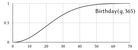
With only people, the probability of a shared birthday is just above 50 percent. The graph could be extended to the right (all the way to ), but even at the probability already exceeds 99.9 percent.
The birthday paradox lived up to expectation at the 2014 FIFA World Cup in Brazil. Each team consisted of twenty-three players, meaning that the probability of a shared birthday in any particular team was , roughly 50 percent. (We are conveniently assuming that birthdays are uniformly distributed, and that February 29 doesn't exist.) Indeed, exactly half of the teams (16 of 32) contained a shared birthday among their players.
Asymptotic bounds: The exact formula for is cumbersome. It is much more convenient to use the following approximations:
For all and :
You remember that , right?
To prove the upper bound, we use the fact that when and are positive,
More generally, when all terms are positive, . Hence,
Applying that fact,
Next, to prove the lower bound, we use the fact that when ,
This fact is illustrated below. The significance of is that
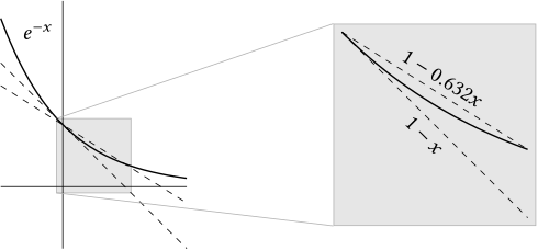
We can use both of these upper and lower bounds on to show the following:
With the last inequality we used the fact that , and therefore (this is necessary to apply the inequality ). Hence:
This completes the proof.
Below is a plot of compared to these upper and lower bounds (for ):
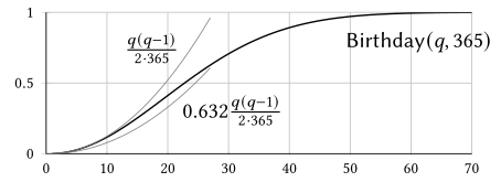
When taking repeated samples from a set of items,
-
Concretely: The probability of a repeat after samples is roughly 0.63. If then .
-
Asymptotically: When the number of samples is much smaller than , the probability of a repeat is roughly . In particular, when is polynomial function of , and an exponential function of , is negligible.
We can express the birthday bound using libraries, which makes it convenient to use in a security proof:
The following two libraries are indistinguishable:
Here, denotes the set of all -bit strings, excluding those in the set . samples from to guarantee that never returns the same value twice.
The proof is a simple application of the bad-event lemma. It uses the fact that is negligible, when is any polynomial.
In some security proofs we can use lemma 4.5.7 to avoid explicitly reasoning about bad events. However, bad events cannot always be avoided, especially when they involve values chosen by the adversary.
Exercises
-
Suppose that and are negligible functions. Prove that and are negligible.
-
Suppose is a negligible function and is a polynomial. Prove that is negligible.
-
For any integer , define the function
-
Prove that for each , is a negligible function.
-
Consider the sum of many 's, where the number of terms in the sum depends on :
Show that is not negligible.
-
Our convention is that all libraries have access to the security parameter as a global variable. For every integer , define the following library:
:if :returnelsereturnProve that for all integers , we have . Remember, we are fixing and the considering the asymptotic behavior of of , as approaches infinity.
-
With defined as above, is ? In this question, the parameter is growing along with the security parameter .
-
-
Prove that the following two libraries are indistinguishable:
:if :returnelse:return:if :returnelse:return:if :returnelse:return:if :returnelse:returnLet's call arguments to a “-values” and arguments to b “-values.” Library checks for repeats among the -values and repeats among the -values. Library checks whether there is any repeat among any combination of -values and values of the form , where is a global secret.
-
Prove that the following two libraries are indistinguishable:
:if undefined or :returnelse: //return:returnIn , the subroutine returns if called twice on consecutive inputs that xor to . It uses to store the previous input to .
-
Prove that the following two libraries are indistinguishable:
:if or :returnelse: return:returnIn , each call to involves an -value (chosen by the adversary) and a -value (uniformly sampled, and secret). It returns if any -value matches any -value (possibly from different calls to ).
-
Prove that the following two libraries are indistinguishable:
:return:return:return:returnIn , the two subroutines will never output a common value, although each subroutine can repeat a value individually.
-
Prove that the following two libraries are indistinguishable:
:return:dountilreturnEach call to takes as input and gives as output. In , it is guaranteed that never repeats.
-
Prove that the following two libraries are indistinguishable:
// is a set of strings:return// is a set of strings:returnAssume that the set is passed as an explicit list. That is, if the calling program runs in polynomial time, then can have only polynomially many items.
Chapter Notes
Although concrete, quantitative treatments of provable security appeared previously and implicitly, the modern concrete approach was pioneered and explicitly advocated in the work of Bellare and Rogaway, together with several groups of coauthors, during the mid-1990s [20,18,15].
The monetary costs in example 4.1.1 were estimated as follows. At the time of writing, the cheapest class of CPU on Amazon's EC2 cloud computing platform that is suitable for a CPU-bound brute force computation is c6g.medium, which is a 2.5 GHz CPU that performs clock cycles per hour. The cheapest rate that I was able to find for this CPU is 0.0157 USD per hour. Thus, the cost for a single clock cycle is roughly USD. The monetary value for “all of human economic activity” is based on estimates of historical gross world product (GWP), due to J. Bradford DeLong [81], combined with more recent modern GWP data.
The estimate of total Bitcoin hashing in example 4.1.2 is based on historical data obtained from blockchain.info.
The extremely unlikely outcomes for casino games in example 4.1.3 are taken from an excellent video by Matt Parker (https://youtu.be/8Ko3TdPy0TU). For more information about the record for most consecutive craps rolls, see: [131].
Definition 4.1.6 is a folklore definition of “-bit security,” although it does not apply equally well to both search (e.g., key recovery) and decision (e.g., distinguishing two libraries) problems. Micciancio and Walter discuss the subtleties of “bit security” and propose a proper formalization [162].
In the modern approach to cryptography, we define security by considering the computational difficulty of attacks, not the total absence of attacks in principle. The earliest hints this approach can be found in the pioneering work of Claude Shannon from 1949 [201]:
Although it is always possible in principle to determine these solutions (by trial of each possible key for example), different enciphering systems show a wide variation in the amount of work required. A good practical secrecy system is one in which the [amount of work needed to break it] remains sufficiently high to prevent the enemy from actually carrying out the solution, or to delay it to such an extent that the information is then obsolete.
Later in 1955, the famous mathematician and economist John Nash sent several letters to the United States National Security Agency (NSA) regarding cryptography. What is notable about Nash's letters is that he explicitly identifies the importance of asymptotic running time (how the cost scales with increasing key sizes) and makes a qualitative distinction between polynomial-time computations as “feasible” and exponential-time computations as “infeasible.”
So a logical way to classify enciphering processes is by the way in which the computation length for the computation of the key increases with increasing length of the key. This is at best exponential and at worst probably a relatively small power of [the key length] , or , as in substitution ciphers.
These remarks are almost a decade ahead of their time. Polynomial time was eventually adopted in algorithms research as a formal definition for “feasible” computation, but not until the work of Cobham [66] and Edmonds [93] in the mid-1960s. Nash's letters to the NSA were declassified in 2012 and made part of an exhibit at the National Cryptologic Museum [171]. The original handwritten letters can be seen at https://joyofcryptography.com/files/nash.pdf.
It is nontrivial to formally define “polynomial time” in a coherent way for interactive programs like the adversaries in our definition of indistinguishability. Hofheinz, Unruh, and Müller-Quade [123] give a thorough treatment of the issue, including a discussion of why the “obvious” approaches fail. When we consider whether and are indistinguishable, the most important condition is that the combined (and self-contained) programs and both run in polynomial time.
The idea of indistinguishable distributions was first proposed by Yao [220].
Suppose , where the number of hybrids depends on the security parameter. Fischlin & Mittelbach [102] point out important subtleties and pitfalls that arise when attempting to deduce that . Exercise 4.3 is from their paper, and claim 4.3.4 is inspired by their formalization.
The bad-event lemma presented here in lemma 4.4.1 is from Bellare and Rogaway [29,30]. Earlier versions of the bad-event lemma were given by Bellare, Krovetz, and Rogaway [22] and by Shoup [204].
Example 4.5.4 is inspired by a BBC Radio feature about the birthday paradox, by James Fletcher (https://www.bbc.com/news/magazine-27835311).