 The Joy of Cryptography
Post-Quantum Cryptography
Cryptography is built on computational problems that are believed to be hard, like breaking a candidate PRP, factoring large integers, calculating discrete logarithms in elliptic curves, to name a few. But quantum computers can solve some problems faster than classical computers; they change the landscape of hard problems. It is therefore important to understand their consequences on cryptography.
Quantum vs. post-quantum: There are two ways quantum computers can affect cryptography:
-
We can imagine designing and deploying new cryptography that requires a quantum computer. Think of Alice and Bob sending entangled photons to each other. This kind of cryptography is called quantum cryptography; it is extremely limited and requires specialized hardware.
-
We can imagine cryptography that runs on traditional, classical computers, but is designed to be secure even against adversaries who have access to a quantum computer. This kind of cryptography is called post-quantum cryptography.
This chapter discusses only post-quantum cryptography.
Urgency: Scalable quantum computers that pose a serious threat to cryptography do not yet exist, and may not exist for many decades. Still, they are plausible enough to warrant serious attention now, because data encrypted and stored today could be decrypted by a future quantum adversary.
Fortunately, paranoia is a virtue in cryptography, and cryptographers like to prepare for the worst-case scenario. Since 2017, NIST has been organizing a process to develop and select new post-quantum cryptographic standards. In 2022, four algorithms (one KEM and three signature schemes) were chosen as future standards. Section 20.3 describes some greatly simplified aspects of the winning KEM design.
20.1. Capabilities of quantum computing
Which problems are easier to solve on a quantum computer? This section summarizes known results that are relevant to cryptography. I will not attempt to describe how quantum computers work, or how these algorithms work; that is well beyond the scope of this book.
20.1.1. Attacking symmetric-key cryptography
Quantum computers can speed up brute-force searches from time to time, using a method called Grover's algorithm:
Let be a function. There is a quantum algorithm, called Grover's algorithm, that makes only quantum evaluations of and outputs a value such that , if any such exists.
You can think of Grover's algorithm as a faster method for finding needles in haystacks. The haystack is , and the needle is the special input that causes to output 1. Grover's algorithm can be used to attack symmetric-key cryptography by applying it to a suitable needle-identification function .
For example, a quantum computer can break an SKE scheme in the following way: First, obtain a few ciphertexts with known plaintexts:
There need to be enough samples so that, with high probability, only one value of is consistent with them all. Usually a very small value of is sufficient. Next, define the following function :
This function checks whether a candidate is consistent with all of the pairs, which are hard-coded as constants into the algorithm's description. By design, there is likely only one value of that causes to output 1, and Grover's algorithm can find it in time .
Grover's algorithm speeds up brute-force attacks, but they remain exponential-time. Additionally, Grover's algorithm is inherently sequential — it cannot be obviously parallelized like a classical brute-force search. The threat of Grover's algorithm can be neutralized by simply doubling the length of the keys. To ensure that quantum brute-force attacks require effort, we can choose keys that are bits long. Of course, this defense helps only if brute-force attacks are the best possible attack. For many symmetric-key primitives, this is assumed to be case; however, it is not true for asymmetric-key primitives.
20.1.2. Breaking asymmetric-key cryptography
In 1994, Peter Shor struck fear into the hearts of cryptographers everywhere by demonstrating that quantum computers could break most asymmetric-key cryptography in polynomial time:
There are quantum algorithms for the following tasks, whose running time is polynomial in :
-
Factoring -bit numbers.
-
Solving the discrete logarithm problem in any cyclic group of order , even groups based on elliptic curves.
Both algorithms use a common approach called Shor's algorithm.
All of the public-key cryptography that you've seen so far relies on either the hardness of factoring (as in RSA) or the discrete logarithm problem (as in Diffie-Hellman, El Gamal, Schnorr signatures). A quantum computer of reasonable size could break all of these schemes. New techniques are needed for post-quantum secure public-key cryptography.
20.2. The learning-with-errors problem
If you were asked to solve for the unknown 's in the following system of equations, your task would be relatively easy:
You can write these as a single matrix equation, then solve it by inverting the square matrix that appears:
This problem is not made any harder by increasing the number of constraints (the height of this matrix), although in this case not every left-hand-side will have a solution. These systems of linear equations can also be solved modulo , as long as the matrix is invertible mod .
Now suppose you are asked to solve a system of approximate equations:
Here, means that the two sides differ by only a very small amount – say, . Such a system of approximate equations is much harder to solve.
We can rewrite these approximate equations as exact equations by introducing an error vector:
Here, the error vector is , whose entries are known to be “small” (say, from ) but are otherwise unknown.
Equations like the one above are useful for cryptography because of the following dichotomy:
-
When the number of approximate equations is high (the matrix is tall), there is generally at most one possible solution in the unknown 's and 's.
-
On the other hand, it appears to be very hard to find that solution or to even determine whether one exists. All known algorithms for this problem, even quantum algorithms, require exponential time.
This chapter uses linear algebra; for a review, see section A.6. Matrices are written as capital bold letters: . Vectors are written as lowercase: . All vectors are column vectors by default, and made into row vectors by taking their transpose .
Learning With Errors: Learning with errors (LWE) is a cryptographic problem based on approximate linear equations of this kind. An adversary is given a matrix and a vector , where is sampled uniformly and is sampled from a distribution of “small” values. All arithmetic is performed modulo .
An output of this LWE process is “close” (within a small error vector) of a vector of the form . If is much taller than it is wide, not every is close to a vector of the form , so not every is a possible LWE output. However, it is believed to be hard to determine whether a has this property. Thus, the LWE assumption is that is indistinguishable from a uniformly distributed vector.
The vector in LWE is called the noise vector. Each component of is sampled independently from a distribution on “small” values, so we call vectors from this distribution “short.” Since we are working mod , instead of thinking about “small” values, think “close to 0,” in either direction. For example, is “small” because . In general, for the purposes of LWE it is helpful to think of not as but as .
The LWE problem is not particularly sensitive to the precise distribution of noise elements; two common choices are a [discretized] Gaussian distribution (normal distribution) and a uniform distribution over for some small .

Consider the following parameters:
-
: the length of the secret (width of matrix).
-
: the number of approximate equalities (height of matrix).
-
: the modulus.
-
: the distribution over noise elements.
The learning with errors (LWE) assumption is that the following libraries are indistinguishable, even to quantum adversaries:


Why “learning” with errors? The secret vector defines a function . The adversary learns input/output samples of this function, one for each row of and , but with added errors/noise.
LWE Security and Parameters: The security of LWE depends on a reasonable choice of the parameters listed above. The choice of these parameters is not as straightforward as it is for, say, RSA. There is not a one-size-fits-all recommendation, because different LWE-based constructions require matrices of different sizes, and are affected differently by the LWE noise. However, the following suggestions can give you a rough sense for the size of the numbers involved, for basic applications of LWE:
-
The secret length should be the security parameter .
-
The modulus should be approximately .
-
The noise distribution should produce outputs bounded in magnitude by approximately .
Using these parameters, the LWE assumption is believed to hold for any parameter (polynomial in the security parameter), even against quantum adversaries!
LWE With Short Secrets: The primary secret in LWE is a uniformly sampled vector. Interestingly, the hardness of LWE does not change if is instead sampled from the noise distribution:
If the LWE assumption is true, then it is also true (with mostly the same parameters) when the secret is sampled from the noise distribution. That is, the following two libraries are indistinguishable:
Consider the following library . It first obtains a standard LWE sample (generated with a uniform secret vector) of dimension , from an external subroutine that we will write as . It uses this LWE sample to generate a new sample of dimension as follows:
This library contains one (intentional) bug: Its behavior is undefined when is not an invertible matrix. For now, let's continue as if is always invertible; then at the end of the proof we will discuss how to be more careful about this step.
With this in mind, we will show that:
Step (2) follows directly from the standard LWE assumption, so we focus on steps (1) and (3). First, no matter which library is linked to, is distributed uniformly and independent of , causing to be distributed uniformly.
When is linked to , the output of has the following structure:
where are sampled from the noise distribution. Then:
So has the structure of an LWE output, where — which is sampled from the noise distribution — now plays the role of the LWE secret. Since and are independent of each other and of , the output of exactly matches that of and we have (1).
When is linked to , is distributed uniformly and independent of . Hence, acts like a variant of OTP using vector addition, where plays the role of OTP key. So is distributed uniformly, and the output of matches that of and we have (3).
When is sampled uniformly, it is indeed highly likely to be invertible. Unfortunately, the probability that fails to be invertible is not negligible. To deal with this problem, we change how generates . Instead of taking rows directly from the LWE sample, take a collection of rows (requiring a standard LWE sample of dimension now), then throw away any of these rows that are linearly dependent of the ones above it. It can be shown that, except with negligible probability, this process results in rows remaining—in other words, an invertible matrix.
20.3. Key exchange from LWE
In this section we discuss how LWE can be used for key exchange. The goal is not to show a realistic protocol (as you will see, the protocol we construct is impractical), but rather to merely provide some basic intuition for applying LWE to public-key cryptography.
Big Picture: Inspired By Diffie-Hellman: The heart of Diffie-Hellman KE is that there are two ways to compute the expression :
Additionally, Alice can send , and Bob can send , because these values “hide” and from an eavesdropper in some way.
LWE-based key exchange is motivated by two different ways to compute a vector-matrix-vector product:


Here, is a public matrix, and and are vectors, so that the product a single scalar. The names are chosen to be suggestive of Diffie-Hellman. Suppose Alice and Bob sample secret vectors and , then Alice sends and Bob sends . Both users could compute the common value in their own way, using the observation above. Would the resulting KE protocol be secure?
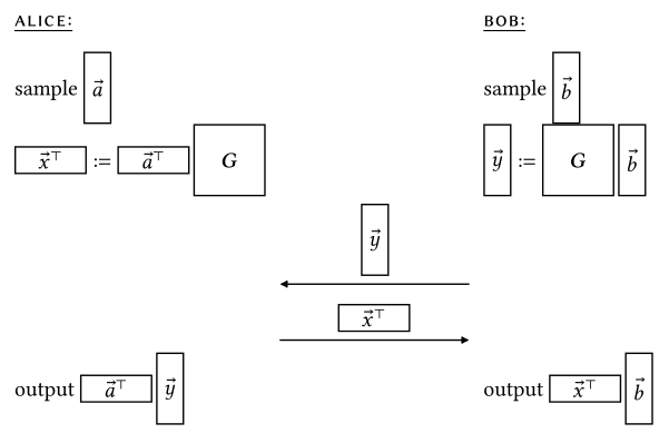
Unfortunately not: The protocol messages and do not hide the secret vectors and in the same way that and hide exponents and in DHKE. However, the LWE assumption suggests that Alice and Bob can hide and by adding noise!
Adding noise: If both Alice and Bob add standard LWE noise to their protocol messages, we obtain the following KE protocol:
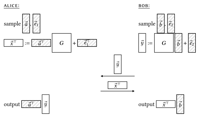
“Short” vectors sampled from the noise distribution are drawn here as shaded boxes. Thanks to lemma 20.2.2, it is safe for both users to sample their secret LWE vectors ( and ) from the noise distribution. We use this fact later.
The two protocol messages each have the form of an LWE vector, which suggests that they hide and . Keep in mind that Alice's protocol message is simply the transpose of a standard LWE vector (using as the LWE matrix):
Although noise is vital for security, it undermines the agreement aspect of key exchange. Alice will compute output:
whereas Bob will compute output:
Their outputs differ by an error amount:
Each vector in this expression (, , , ) is a short vector, sampled from the noise distribution. It is possible to choose secure parameters for the noise distribution, to ensure that is sufficiently small: Say, is negligible. The quantitative analysis is tedious, and beyond the scope of this book. But the conclusion is that Alice and Bob compute values that may not be identical, but are certainly close.
Reconciliation: Alice and Bob now hold values in that are within distance . You can visualize the situation as follows, where we list the elements of in a circle, like the face of a clock.
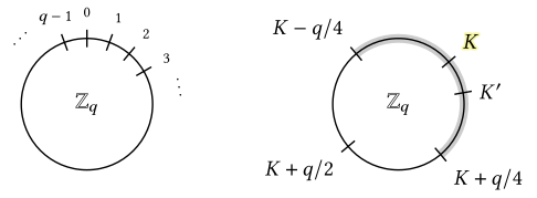
Call Alice's value and Bob's . In the diagram above, Alice doesn't know Bob's but she knows that it is always in the shaded region.
To convert their approximately equal values into truly equal values, Alice can uniformly sample a bit and send the message to Bob. In other words, if , then Alice sends , which is very close to Bob's ; If then Alice sends a value that is diametrically opposite in the circle, and therefore more than away from Bob's . Bob can easily distinguish these two cases, and thereby learn . Finally, Alice and Bob can agree on a common value! But an eavesdropper will not learn because, as we will show, is pseudorandom to an eavesdropper, and acts as a one-time pad to mask .
Careful readers will have noticed that Alice and Bob have gone to all this work only to agree on a single bit! This is true, and this is what makes the protocol impractical. In principle, Alice and Bob could run parallel instances of this protocol, to agree on a -bit key, but this would be incredibly expensive. Real-world LWE-based KE protocols are much more efficient, and we will briefly discuss them later. Still, they are based on the core ideas from this simplified protocol.
The protocol that results from this discussion is presented below. For reasons that shall become clear in the security analysis, Alice must add a noise term to her value of .
Let , , and be suitable LWE parameters. A key exchange protocol based on LWE is the following:
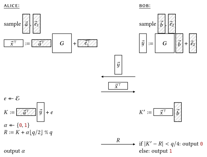
Of course, the final two protocol messages (from Alice to Bob) can be sent together as a single message.
The matrix can be sampled by one of the users and included in the first protocol message. Alternatively, it can be global, and reused across several instances of the protocol, as long as it has been sampled uniformly.
Construction 20.3.1 is a passively secure KE protocol if the LWE assumption holds.
LWE-based key exchange in practice: This KE protocol has been presented as a glimpse into the general techniques of post-quantum cryptography. As you saw, it is far from practical and requires considerable effort to agree on just a single bit.
In 2024, NIST standardized a new post-quantum PKE/KEM scheme called ML-KEM. It is based on the LWE approach described in this chapter but offers better performance through a few techniques:
-
Our simple KE protocol has throughput of one bit because it is based on a vector-matrix-vector multiplication expression that results in a single scalar value. However, it is also possible to design a KE protocol based on matrix-matrix-matrix multiplication, which will allow Alice and Bob to (approximately) agree on an entire matrix of values. Exercises 20.4 and 20.7 give a roadmap to such a construction.
-
Standard LWE involves a uniformly chosen matrix, but there exist LWE variants in which the matrix has some additional algebraic structure. For example, in the ring LWE variant, the matrix is not arbitrary but is built from blocks, where each block has the special form:
Matrices of this form offer a few benefits: First, each block is entirely determined by its first row, meaning that it is times cheaper to communicate these kinds of matrices in a protocol. Second, there are more efficient algorithms for multiplying these special kinds of matrices.
Exercises
-
Explain how to break a PRG in time on a quantum computer. Clearly describe an attack and analyze its distinguishing advantage.
-
This exercise develops a quantum algorithm for finding collisions in a hash function.
-
Using an analysis similar to lemma 4.5.5, show that the following program has at least a 50 percent chance of outputting when :
-
Let be a random oracle with output bits. We will write inputs to as integers rather than strings. Consider the following quantum algorithm for finding a collision in . What is the probability that it successfully finds a collision, and what is its running time?
-
-
Let be parameters for the LWE problem. Suppose for the sake of simplicity that the error distribution outputs values from the range .
-
With these parameters, how many outputs are possible from lwe.sample in ? (definition 20.2.1)
-
With these parameters, how many outputs are possible from lwe.sample in ?
-
Suppose we use the suggested parameters , , and . How do your answers to (a) and (b) scale with and , especially when is much larger than ?
-
-
In this exercise, we extend LWE secrets from vectors to matrices. Prove that if the LWE assumption is true for parameters , then for any parameter the following two libraries are indistinguishable:
:return:return -
Formally show that the warmup protocol shown in the first figure in section 20.3 is not a passively secure KE protocol.
-
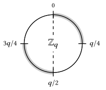
In construction 20.3.1, Alice and Bob exchange a single scalar that helps them agree on an output bit . Consider the following approach that works when is a multiple of 4, and the noise (difference between and ) is bounded by . Alice sends a only single bit, indicating whether her value of is in the shaded region below; both users output a bit indicating whether Alice's is left or right of the dashed line.
-
Explain/prove why the bit sent by Alice leaks nothing about the output bit.
-
Explain how Bob can output the same secret bit as Alice.
-
-
Using exercise 20.4 as inspiration, design a KE protocol in which the two parties agree on bits, after exchanging elements of ( is the LWE parameter). Prove that your protocol is secure.
-
Propose a PKE scheme based on construction 20.3.1 and prove that it is CPA-secure under the LWE assumption. Your scheme can support single-bit plaintexts.
-
There are variants of LWE that are unconditionally secure. For example, if the matrix is sufficiently wide () and the secret vector is sampled not from but from , then the resulting LWE variant is secure, without any noise! In other words, the following two libraries are indistinguishable:
:return:returnIn section 20.3 we develop a KE protocol starting from the idea that , but where both users add LWE noise to their vectors.
-
Design a KE protocol in which one participant adds noise, but the other uses this noiseless LWE variant. Identify the error term (difference between users' approximately-equal values), and prove that your protocol is secure.
-
Propose two different PKE schemes based on this KE protocol, and prove that they are CPA-secure. The participants in the KE protocol have asymmetric roles, and the two PKE schemes arise by assigning different participants to the roles of ciphertext and public key.
-
Chapter Notes
For an accessible and nontechnical summary of limitations of quantum (not post-quantum) cryptography, see the recent report from several European government agencies [103].
Grover's algorithm is named for its creator, Lov Grover [117]. The collision-finding algorithm in exercise 20.2 is due to Brassard, Høyer, and Tapp [54]. There is debate as to whether this quantum algorithm could ever be more efficient than the classical birthday attack (see Bernstein [36]).
Shor's algorithm is named after its creator, Peter Shor [202].
The learning with errors assumption was introduced by Regev [188]. Claim 20.2.2 is due to Applebaum, Cash, Peikert, and Sahai [6]. For a comprehensive overview of LWE and lattice-based cryptography in general, see the retrospective article by Peikert [179].
The ML-KEM standard is based on the Kyber KEM, of Avanzi, Bos, Ducas, Kiltz, Lepoint, Lyubashevsky, Schanck, Schwabe, Seiler, and Stehlé [8].
Construction 20.3.1 is based on the PKE schemes of Lyubashevsky, Palacio, and Segev [151] and Lindner and Peikert [148]. The two approaches suggested in exercise 20.9 give rise to well-known PKE schemes: the one proposed by Regev in the paper that introduced the LWE assumption [188] and the “dual-Regev” scheme proposed by Gentry, Peikert, and Vaikuntanathan [109]. These use a noiseless variant of LWE based on a result called the leftover hash lemma, which is due to Impagliazzo and Zuckerman [125]. The noise-reconciliation method of exercise 20.6 is due to Peikert [178].